Tutorials
Hopkins & Skellam established in 1954 the Hopkins statistic to assess the global clustering tendency of a dataset by testing its spatial randomness through quantitative measurements of its uniformity. A single global value is calculated through a comparison of the mean k-nearest neighbour distances between objects within the dataset, and between points in the dataset and a similarly constructed uniform random sample.
INDICATE (INdex to Define Inherent Clustering And TEndencies) is a novel statistical clustering tool tool to assess and quantify the degree of spatial association of an object in a dataset. Highly versatile, INDICATE has many applications, including characterising morphological stellar features and tracing spatial evolution in star forming regions.
References:
- Hopkins, B., & Skellam, J. G. (1954). A new method for determining the type of distribution of plant individuals. Annals of Botany, 18(2), 213-227.
- Buckner, A. S., Khorrami, Z., Khalaj, P., Lumsden, S. L., Joncour, I., Moraux, E., ... & Herrera-Fernandez, J. M. (2019). The spatial evolution of young massive clusters-I. A new tool to quantitatively trace stellar clustering. Astronomy & Astrophysics, 622, A184.
- Buckner, A. S., Khorrami, Z., González, M., Lumsden, S. L., Moraux, E., Oudmaijer, R. D., ... & Hacar, Á. (2020). The Spatial Evolution of Young Massive Clusters II. Looking for Imprints of Star Formation in NGC 2264 with Gaia DR2. Astronomy & Astrophysics, 636, A80.
- The INDICATE source can be found at: https://github.com/abuckner89/indicate
The input parameters of this algorithm are:
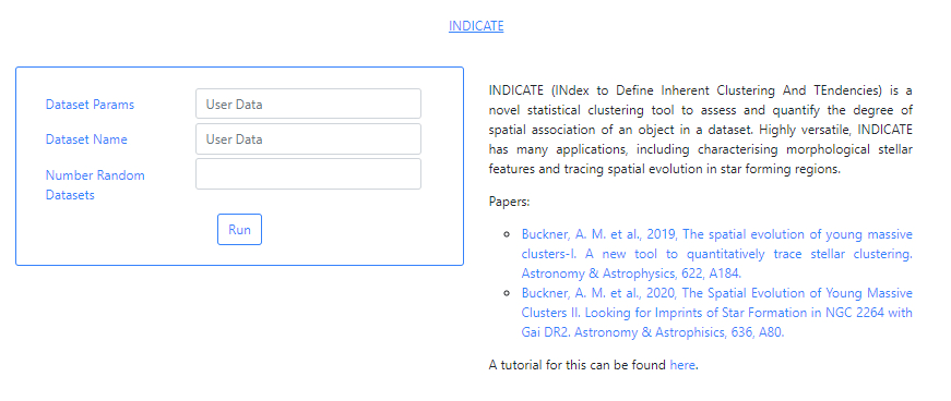
Dataset Params: A CSV file containing the parameters of the dataset. The file should contain a single row per dataset with the following columns:
Dataset Name min(X) max(X) min(Y) max(Y) Surface Area Note that the surface area should be given as a unitless float for 2D datasets.
Dataset Name: A CSV file containing the positions of the data points corresponding to Dataset Name. Each row should contain two columns with the X, Y position of a single data point. Columns give position in each axis, i.e.,
Number Random Datasets: The algorithm needs to generate a number of randomly distributed dataset of the same size as Dataset Names and in the same parameter space. This number is a positive integer.
| X | Y |
For this tutorial, we provide some files that can be downloaded to illustrate the usage of INDICATE, INDICATE_DEAVI_example.zip. Once the file is downloaded, unzip the file. The file INDICATE_DEAVI_example.zip contains two files that can be uploaded into the different fields of the input parameters interface of INDICATE. The two files are:
Dataset Params file: dataset_s1_params_2D.csv. This file contains the following information in a single line with comma separated values:
s1,19835,961951,51121,970756,866402847660
which correspond to:
| Dataset Name | min(X) | max(X) | min(Y) | max(Y) | Surface Area |
|---|---|---|---|---|---|
| s1 | 19835 | 961951 | 51121 | 970756 | 866402847660 |
Dataset Name: dataset_s1.csv. The file provides the X, Y values for each data point in the dataset. In this particular case, this file contains 5000 data points.
In order to upload these two files to DEAVI, go to the File Manager section inside the Data tab and navigate to /home/user. Every user has a specific area to upload any files needed by the algorithms. Click on the File Select icon.

A window will appear to access and select files in your computer. Select the file dataset_s1_params_2D.csv. Once the file is selected, the name of the file will appear in the same icon.

Then click the file icon to the right of the box showing the name of the file to be uploaded.
Upload in the same manner the file dataset_s1.csv.
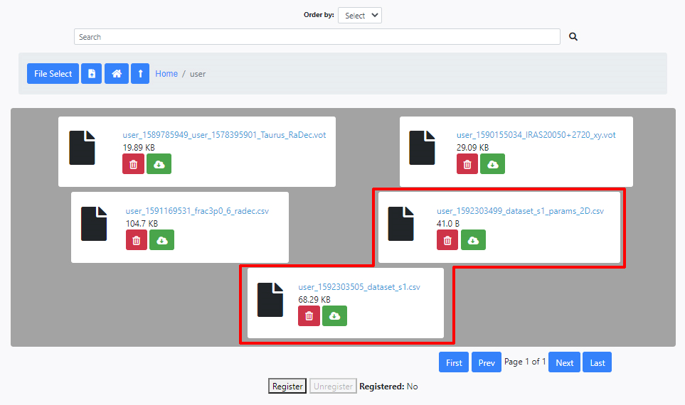
Both files are now available and can be loaded into the input parameters interface of INDICATE. A Unique Identifier is added to every file when they are uploaded to avoid overwriting files. The image below shows a typical user file area with some files, including the two just uploaded. The files can be deleted or downloaded from here.
We can now go back to the INDICATE algorithm and upload these two files. Simply typing user in the Dataset Params and Dataset Name fields will bring a drop-down menu from which the files can be selected. For this particular example we use 10 Random Datasets.
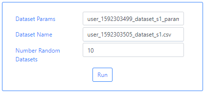
Finally, the user can launch the algorithm by clicking on the Run button.
Once launched, the user is redirected to the Pipeline Status section of the Algorithms tab. A message appears saying that the algorithm has started. Also, under the Status column, the message STARTED appears. At this point, the execution can be aborted by clicking the Abort button to the right of the panel. This algorithm can take some time to finish its execution.

Once finished, the Status column is changed to SUCCESS if the algorithm has run successfully. At this point, the execution can be deleted by clicking the Delete button to the right of the panel.

By clicking in the arrow close to the name of the algorithm in the Name column, the results panel is opened.
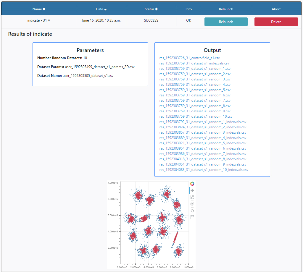
Three panels appear:
- Parameters: here the list of input parameters used in this particular execution of the algorithm is displayed.
- Output: Any outputs produced by the algorithm are shown here. In this case a list of ascii files is displayed, in particular 10 pairs of files and two auxiliary files, as indicated by the input parameter Number of Random Datasets. The contents of the files can be explored by clicking on their names. The results of the execution can also be found in the File Manager section of the Data tab. The files are stored under /Home/results.
- Plots panel: Any plots produced by the algorithm are displayed here. In this case, the output of INDICATE. All the plots allow some degree of interaction by using the panel in the top right-hand side. The functionalities allow to zoom, pan and save the plots.
S2D2 is an algorithm that uses the Density-Based Spatial Clustering of Applications with Noise (DBSCAN) to detect the smallest significant structure in a spatial/spatial-kinematic space. The procedure proposes, in structured regions, the calculation of the epsilon scale and Nmin parameters for DBSCAN to retrieve the smallest structures in the region with a 3-sigma level significance. If the region is not structured, or the user wants it, epsilon scale and Nmin can be supplied, and DBSCAN will be run with the user defined parameters, however, without guaranteeing any level of significance.
References:
- González, M. et al (2020). ‘S2D2: Small-scale significant substructure DBSCAN Detection. I. NESTs detection in 2D star-forming regions’, A&A, 647, A14.
- Joncour I., Duchêne, G., Moraux, E., ‘Multiplicity and Clustering in Taurus star-forming region. I. Unexpected ultra-wide pairs of high order multiplicity in Taurus’, 2017, A&A, 599.
- Joncour I., Duchêne, G., Moraux, E., Motte, F. ‘Multiplicity and Clustering in Taurus star-forming region. II. From ultra-wide pairs to dense NESTs’, 2018, A&A, 620.
The input parameters of this algorithm are:
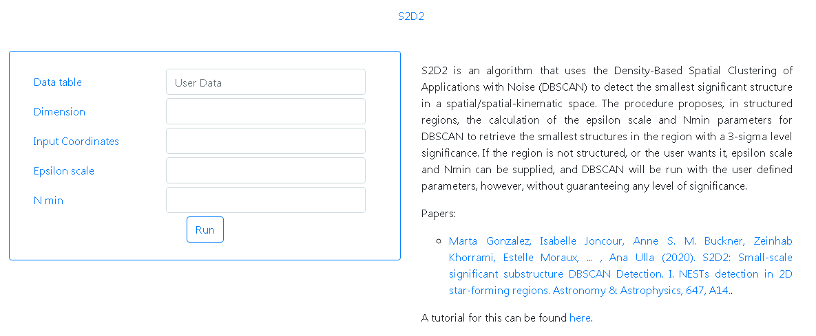
-
Data table: VOTable user uploaded file containing the coordinates of the objects. The file must contain the columns named accordingly to the input coordinates: 'ra' and 'dec' for celestial coordinates and 'x' and 'y' for rectangular.
-
Dimension: A string corresponding to the dimension of the analysis. Only '2D' (without quotes) is accepted for now.
-
Input Coordinates: A string indicating the type of input coordinates. Only 'ra dec' for celestial coordinates or 'x y' (without quotes) are valid for the 2D dimension.
-
Epsilon scale: Float. This is the Epsilon parameter for the DBSCAN algorithm. A value of 0 is recommended, for the smallest scale calculation. If supplied, N min must also be supplied, in which case, just DBSCAN will be performed.
-
N min: Integer. This is the minimum number of points for DBSCAN. The recommended value is 0, for significant density calculation. If supplied, Epsilon scale must also be supplied, in which case, just DBSCAN will be performed.
For this tutorial, we provide a file that can be downloaded to illustrate the usage of S2D2, Taurus_RaDec.vot. Once the file is downloaded to a local folder, it has to be uploaded into DEAVI.
In order to upload these two files to DEAVI, go to the File Manager section inside the Data tab and navigate to /home/user. Every user has a specific area to upload any files needed by the algorithms. Click on the File Select icon.

A window will appear to access and select files in your computer. Select the file Taurus_RaDec.vot. Once the file is selected, the name of the file will appear in the same icon.

Then click the file icon to the right of the box showing the name of the file to be uploaded.
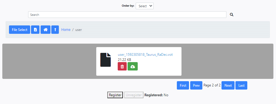
The file is now available and can be loaded into the input parameters interface of S2D2. A Unique Identifier is added to every file when they are uploaded to avoid overwriting files. The image below shows a typical user file area with the uploaded file. The file can be deleted or downloaded from here.
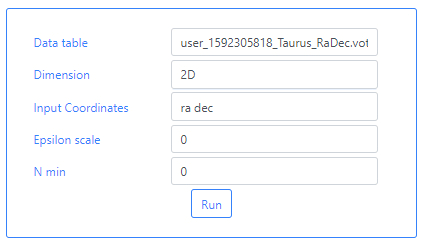
We can now go back to the S2D2 algorithm and upload this file. Simply typing user in the Data Table field will bring a drop-down menu from which the file can be selected. For the rest of the parameters, the image below shows the values to be used. For this particular example we use Epsilon scale and N min equal to 0.
Finally, the user can launch the algorithm by clicking on the Run button.
Once launched, the user is redirected to the Pipeline Status section of the Algorithms tab. A message appears saying that the algorithm has started. Also, under the Status column, the message STARTED appears. At this point, the execution can be aborted by clicking the Abort button to the right of the panel. This algorithm can take some time to finish its execution.

Once finished, the Status column is changed to SUCCESS if the algorithm has run successfully. At this point, the execution can be deleted by clicking the Delete button to the right of the panel.

By clicking in the arrow close to the name of the algorithm in the Name column, the results panel is opened.
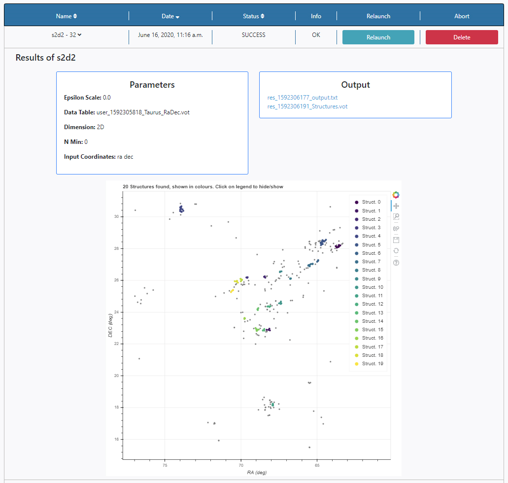
Three panels appear:
-
Parameters: here the list of input parameters used in this particular execution of the algorithm is displayed.
-
Output: Any outputs produced by the algorithm are shown here. In this case:
- XXX_output.txt: Text file where the general results of the process (Q parameter, region density, epsilon, N min, number of structures found) and progress of the algorithm will be recorded.
- XXX_Structures.vot: VOTable file, where the input coordinates and an additional column indicating the small-scale structure to which each object belongs. The tag indicating the structure follows python’s convention, so detected structures are numbered from 0 onwards, and noise corresponds to - 1.
- XXX_errors.txt: Text file where input errors, if any, will be output.
The contents of the files can be explored by clicking on their names. The results of the execution can also be found in the File Manager section of the Data tab. The files are stored under /Home/results.
-
Plots panel: Any plots produced by the algorithm are displayed here. In this case, the output of S2D2 is a figure showing a map of the region with all the objects displayed as grey dots, and those belonging to a structure in colour. All the plots allow some degree of interaction by using the panel in the top right-hand side. The functionalities allow to zoom, pan and save the plots or by clicking on the legend the colored dots appear and disappear.
Considerations:
The coordinates accepted for the input are:
Celestial coordinates, Right Ascension and Declination. In this case, distances between objects will be calculated using the great circle distance. The input coordinates parameter has to be set to 'ra dec', and the VOTable should contain columns 'x' and 'y'.
Rectangular coordinates, for which the Euclidean distance will be used.
Structured regions: it is considered that a star-forming region is structured when the Q parameter is lower than 0.8. In that case and if the user has provided, as recommended, epsilon = 0 and Nmin = 0 we calculate them and obtain the smallest scale significant structure in the region. For values between 0.7 and 0.8, the user will be warned that the region is close to homogeneous.
Epsilon calculation: Small scale. We calculate the length scale for DBSCAN (epsilon) using the One point correlation function, OPCF, comparing the first nearest neighbor distance distribution of the sample with the first nearest neighbor distance distribution of a homogeneous random distribution (CSR, or complete spatial randomness) with intensity equal to the local density derived from the mean of the 6th neighbor distribution of the sample.
N min calculation: Significant. We iteratively calculate the significance of a structure of that scale and a fixed number of points k until we reach 3-sigma significance (~99.85%). The significance of a structure of size epsilon and k points is given by the probability of having k-1 nearest neighbors in an epsilon neighborhood under a homogeneous random distribution with intensity rho.
DBSCAN detection. We run scikit.learn’s DBSCAN for the previously calculated epsilon and N min.
Unstructured regions: If the Q parameter is larger than 0.8, and the user has not supplied an epsilon and N min, we cannot guarantee that the region is structured and/or the nature of the structures found, so we display it as a message giving a suggestion to the user to try DBSCAN providing epsilon and N min. We run scikit.learn’s DBSCAN for the user defined epsilon and N min.
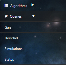
The user can make queries to the Gaia ESA archive by clicking on Gaia.
DEAVI only provides a simple interface to the full Gaia archive. For more information on the use of the Gaia archive or its products please visit the official ESA Gaia archive.
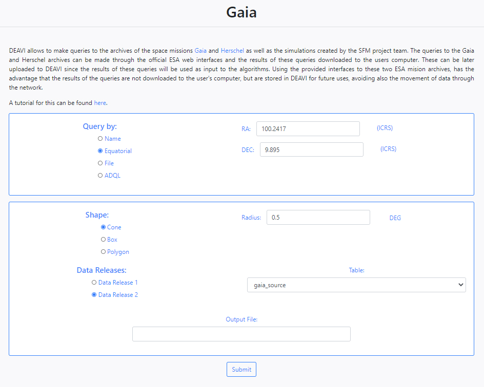
DEAVI implements a help system where by hovering, and in some cases clicking on parameter names, specific help is displayed.
The Gaia query interface in DEAVI provides four different ways of making queries.
- Name
The application allows you to make queries to the Gaia archive by name using the SIMBAD/NED name resolver. For example, if we enter M45, the query to star cluster Messier 45 will be made.
- Equatorial
The default option is search by equatorial coordinates. In this case the user must fill in the parameters of the coordinates Right Ascension (RA) and Declination (Dec). Different coordinate formats are allowed.
When using query by Name or Equatorial, at the bottom of the form, the user must choose the shape of the query (Cone, Box or Polygon),

When the shape of the query is a Cone, the user must enter the value of the radius in degrees. If the option chosen is a Box, the user must enter the height and width in degrees. In the case of a Polygon search, the user must fill in the value of the vertices separated by commas,

Next, the version of the Gaia data (Data Release 1 or Data Release 2) and the Gaia Table to be used in the query search must be selected. Last, a string can be given to be appended to the name of the output file.
- File
DEAVI also provides an option to make queries by uploading a file. To do this, the user must choose the File option and upload the file using the Choose File button that becomes available (depending on the browser this button can have a different caption).

- ADQL
The last available option to make queries is through the use of the ADQL language. By default, choosing this option displays an example query.

When all the parameters of the query form have been filed in, clicking the Submit button at the bottom of the form will launch the query. By clicking on the Submit button, the application will automatically redirect and load the Status table of the Queries section. The results of the query are accessible through the Status table and will also be available through the File Manager in the Data section in the directory /Home/sources/gaia.
Note on using Query by File
In order to use the option of query by File, the file to be uploaded has to have a specific format, in particular, it has to follow the JSON format.
For each desired query, a source_x tag must be inside the, each block with its specific parameters. The example below includes two queries, source_1 and source_2.
                                                                    {"input":{
                                                                       "source_1":{
                                                                       },
                                                                       "source_2":{
                                                                       }
                                                                    }}
Just like when using the form, it is possible to query the Gaia archive by name or coordinates. For example, in the source_1 block, one can input,
-
To query by name:
                                                                            "source_1":{
                                                                               "name": "ngc2264"
}, -
To query by equatorial coordinates:
                                                                            "source_1":{
                                                                               "ra": "100.2417",
                                                                               "dec": "9.895"
                                                                            },
Note that it is possible to use other input formats for ra and dec such as:
"source_1":{
"ra": "06 40 58.000",
"dec": "+09 53 42.00"
},"source_2":{
"ra": "06h40m58.000s",
"dec": "+09d53m42.00s"
},
Regarding the shape, just like in the form, it is possible to make queries with a Cone, Box or Polygonal shape as:
-
Cone:
                                                                                "source_1":{
                                                                                   "shape": "cone",
                                                                                   "radius": "0.5"
}, -
Box:
                                                                                "source_1":{
                                                                                   "shape": "box",
                                                                                   "width": "1",
                                                                                   "height": "0.6"
}, -
Polygon:
                                                                                "source_1":{
                                                                                   "shape": "polygon",
                                                                                   "ra": "10.0",
                                                                                   "dec": "-10.5",
                                                                                   "vertex_1":{ "ra": "20.0", "dec", "20.5"},
                                                                                   "vertex_2":{ "ra": "30.0", "dec", "30.5"}
                                                                                },
To specify the Gaia table to query within a specific Gaia Data Releases,
                                                                "source_1":{
                                                                   "table": "gaiadr2.gaia_source"
                                                                },
Notice that the gaiadr2 must be added before the table's name to query the Data Release 2. To query other data release change it to the correct one.
Last, it is also possible to add a tag to the output files,
                                                                "source_1":{
                                                                   "output_file": "source_1"
                                                                },
The following block shows a completed example of input file for two queries,
                                                                {"input":{
                                                                   "source_1":{
                                                                       "ra": "100.2417",
                                                                       "dec": "9.895",
                                                                       "shape": "cone",
                                                                       "radius": "0.5",
                                                                       "table": "gaiadr2.gaia_source",
                                                                       "output_file": "source_1"
                                                                   },
                                                                   "source_2":{
                                                                       "name": "ngc2264",
                                                                       "shape": "box",
                                                                       "width": "1",
                                                                       "height": "0.6",
                                                                       "table": "gaiadr2.gaia_source",
                                                                       "output_file": "source_2"
                                                                   }
                                                                }}
The user can make queries to the Herschel ESA archive by clicking on Herschel.

DEAVI only provides a simple interface to the full Herschel archive. For more information on the use of the Herschel archive or its products please visit the official Herschel ESA archive.
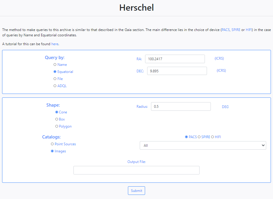
DEAVI implements a help system where by hovering, and in some cases clicking on parameter names, specific help is displayed.
The Herschel query interface in DEAVI provides four different ways of making queries.
- Name
The application allows you to make queries to the Gaia archive by name using the SIMBAD/NED name resolver. For example, if we enter M45, the query to star cluster Messier 45 will be made.
- Equatorial
The default option is search by equatorial coordinates. In this case the user must fill in the parameters of the coordinates Right Ascension (RA) and Declination (Dec). Different coordinate formats are allowed.
When using query by Name or Equatorial, at the bottom of the form, the user must choose the shape of the query (Cone, Box or Polygon),

When the shape of the query is a Cone, the user must enter the value of the radius in degrees. If the option chosen is a BoxM, the user must enter the height and width in degrees. In the case of a Polygon search, the user must fill in the value of the vertices separated by commas,

Next, the version of the Herschel catalogues has to be specified, either Point Sources or Images. If Point Sources is selected a drop-down menu allows to search in a specific catalogue. If Images is selected, an instrument needs to be selected (PACS, SPIRE or HIFI) and a drop- down menu allows to select the product level. Last, a string can be given to be appended to the name of the output file.
- File
DEAVI also provides an option to make queries by uploading a file. To do this, the user must choose the File option and upload the file using the Choose File button that becomes available (depending on the browser this button can have a different caption).

- ADQL
The last available option to make queries is through the use of the ADQL language. By default, choosing this option displays an example query.

When all the parameters of the query form have been filed in, clicking the Submit button at the bottom of the form will launch the query. By clicking on the Submit button, the application will automatically redirect and load the Status table of the Queries section. The results of the query are accessible through the Status table and will also be available through the File Manager in the Data section in the directory /Home/sources/hsa.
Note on using Query by File
In order to use the option of query by File, the file to be uploaded has to have a specific format, in particular, it has to follow the JSON format.
For each desired query, a source_x tag must be inside the, each block with its specific parameters. The example below includes two queries, source_1 and source_2.
                                                                {"input":{
                                                                   "source_1":{
                                                                   },
                                                                   "source_2":{
                                                                   }
                                                                }}
Just like when using the form, it is possible to query the Gaia archive by name or coordinates. For example, in the source_1 block, one can input,
-
To query by name:
                                                                        "source_1":{
                                                                           "name": "ngc2264"
}, -
To query by equatorial coordinates:
                                                                        "source_1":{
                                                                           "ra": "100.2417",
                                                                           "dec": "9.895"
                                                                        },
Note that it is possible to use other input formats for ra and dec such as:
"source_1":{
"ra": "06 40 58.000",
"dec": "+09 53 42.00"
},"source_2":{
"ra": "06h40m58.000s",
"dec": "+09d53m42.00s"
},
Regarding the shape, just like in the form, it is possible to make queries with a Cone, Box or Polygonal shape as:
-
Cone:
                                                                        "source_1":{
                                                                           "shape": "cone",
                                                                           "radius": "0.5"
}, -
Box:
                                                                        "source_1":{
                                                                           "shape": "box",
                                                                           "width": "1",
                                                                           "height": "0.6"
}, -
Polygon:
                                                                        "source_1":{
                                                                           "shape": "polygon",
                                                                           "ra": "10.0",
                                                                           "dec": "-10.5",
                                                                           "vertex_1":{ "ra": "20.0", "dec", "20.5"},
                                                                           "vertex_2":{ "ra": "30.0", "dec", "30.5"}
                                                                        },
Also, the selection of the Catalog is possible,
-
Point Source:
                                                                        "source_1":{
                                                                           "positional_source": "True",
                                                                           "table": "pacs_point_source_070"
                                                                        },
Notice that the positional_source tag must be set at 'True'
-
Images:
                                                                        "source_1":{
                                                                           "positional_source": "Flase",
                                                                           "instrument": "PACS",
                                                                           "level": "level1"
                                                                        },
Notice that the positional_source tag must be set at 'False'
Last, it is also possible to add a tag to the output files,
                                                                "source_1":{
                                                                   "output_file": "source_1"
                                                                },
The following block shows a completed example of input file for two queries,
                                                                {"input":{
                                                                   "source_1":{
                                                                       "ra": "100.2417",
                                                                       "dec": "9.895",
                                                                       "shape": "cone",
                                                                       "radius": "0.5",
                                                                       "positional_source": "True",
                                                                       "table": "pacs_point_source_070",
                                                                       "output_file": "source_1"
                                                                   },
                                                                   "source_2":{
                                                                       "name": "ngc2264",
                                                                       "shape": "box",
                                                                       "width": "1",
                                                                       "height": "0.6",
                                                                       "positional_source": "Flase",
                                                                       "instrument": "PACS",
                                                                       "level": "level1",
                                                                       "output_file": "source_2"
                                                                   }
                                                                }}
The status of all the queries launched from DEAVI can be inspected from the Status section of the Queries tab. Queries are launched from the Submit button available at the bottom of the different query forms provided; Gaia, Herschel and Simulations.
Once queries are launched, DEAVI will automatically load the Status table of the Queries section,
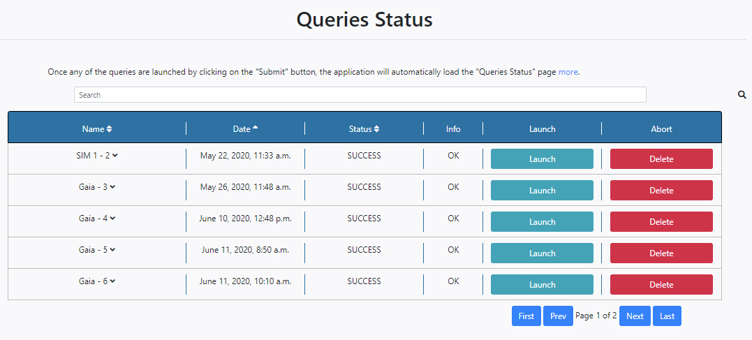
The operations and options available in this panel are self-explanatory and similar to those for the Pipeline Status in the Algorithm tab with some differences:
- The Status column has four possible status: PENDING, STARTED, ERROR and SUCCESS.
- The Launch button on the right of the panel opens up a further Select Algorithm field at the top of the queries with a drop-down menu where it is possible to choose an algorithm that will run over the results of that particular query.
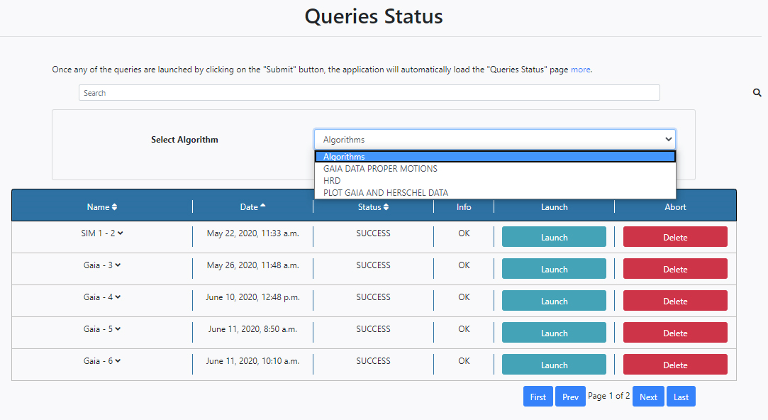
When an algorithm is selected from the drop-down menu, the configuration panel of the chosen algorithm is shown. It is then also possible to configure the algorithm parameters from here and launch the algorithm by clicking Run. In the example shown below the HRD Algorithm is selected and its parameters become available.
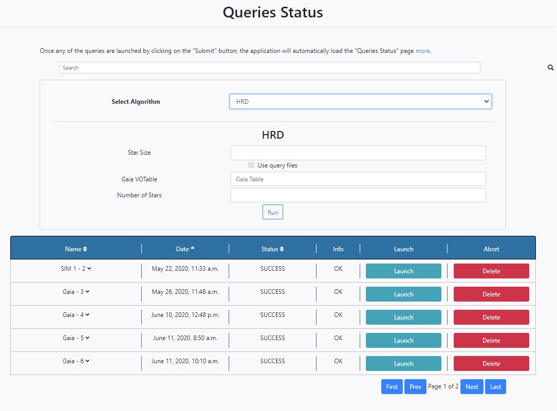
So, it is possible to launch algorithms directly from the Queries Status section.
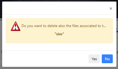
Pressing Delete, will delete the entry from this table. A pop-up window will ask if also the files associated with this query are to be deleted.
The Nbody6 simulation series of star clusters belong to the MYOSOTIS algorithm and they have been performed within the StarFormMapper (SFM) project. For more information about the simulations and/or MYOSOTIS, the following document is available,
http://sims.starformmapper.es/files/Simulation_documentation.pdf
In this tutorial we just highlight the steps to be taken to access the simulation files from DEAVI.
MYOSOTIS
The code MYOSOTIS (Make Your Own Synthetic ObservaTIonS) is designed to produce synthetic observations from simulated clusters. MYOSOTIS can synthesize observations from both ground and spaced-based observatories, for a range of different filters, observational conditions and angular/spectral resolution.
Inputs:
- Stars information (e.g. from Nbody simulations):
- Position, velocity, mass, age, metallicity
- Cloud information (from SPH simulations):
- Particle’s position, mass, smoothing length
- Extinction model and Rv
- OB-treatment: TLUSTY model atmosphere
- Velocity dispersion, for Doppler effect
- Telescope: Filter, resolution, pixel sampling
- Atmospheric condition: Seeing, SR, S/N, contrast and sensitivity
- Euler angles for line-of-sight
Output:
- *_cube_spectra.fits : 3D cube, X-Y is the position of stellar sources, z is flux in different wavelengths
- *_Lambda.txt : the wavelengths [A] which is used for the 3rd dimension of the spectral_cube
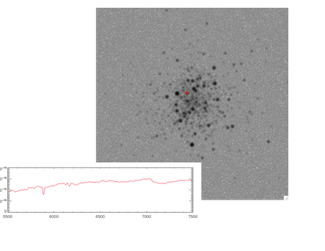
Example Output:
- Gaia-G filter
- R=700
- HST/WFPC2/V
- VLT/SPHERE/Ks
- Example spectra:
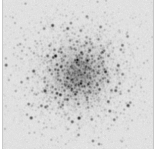
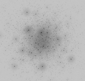
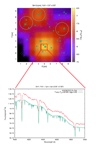
References:
- Khorrami, Z. et al., 2019, A code to Make Your Own Synthetic ObservaTIonS (MYOSOTIS). Monthly Notices of the Royal Astronomical Society, 485(3), 3124-3133.
- The MYOSOTIS source can be found at: https://github.com/zkhorrami/MYOSOTIS
These simulations can be downloaded and used by DEAVI users. For this, you have to click on the Queries tab and then the Simulations section.
The dynamical and stellar evolution of these star clusters have been studied within 100Myr. The required input parameters are:
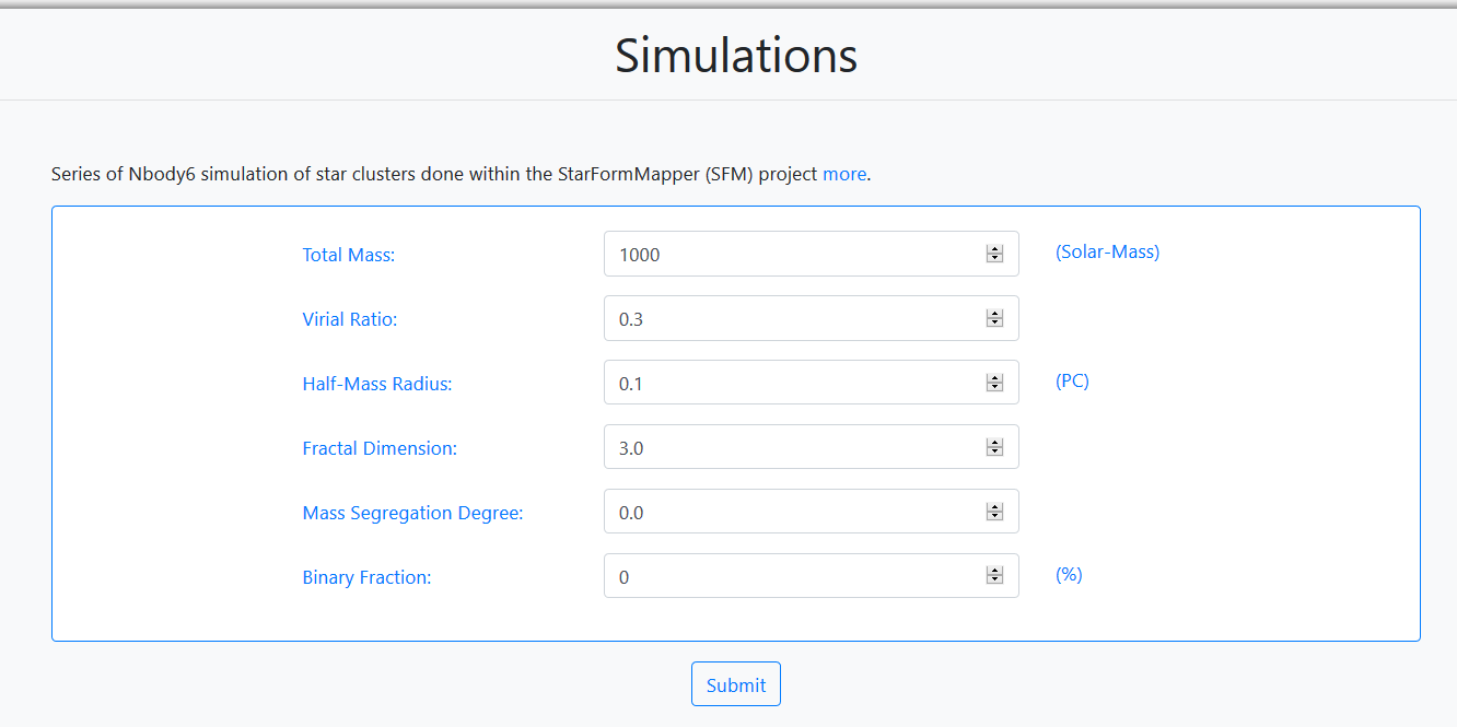
- Total Mass: Total mass of the star cluster. Accepted values are, 10 3 and 10 4 (Solar- Mass).
- Virial Ratio: The virial radius of a gravitationally bound astrophysical system is the radius within which the virial theorem applies. Accepted values are, 0.5 (equilibrium) and 0.3 (collapsing).
- Half-Mass Radius: Half-mass radius of a cluster (units of pc). Accepted values are, 0.1, 0.5 and 1.0.
- Fractal Dimension: Fractal dimension of the data. Accepted values are, 0 (symmetric) and 2.0.
- Mass Segregation Degree: Degree of mass segregation. Accepted values are, 0.0 (no- segregation) and 1.0 (totally segregated).
- Binary Fraction: Binary content of a globular cluster (%).
For this tutorial the values shown in the figure are used for the query. These are the defaults loaded. When all the fields are filled in, the user can launch the query by clicking on the Submit button.
Once launched, the user is redirected to the Status section of the Queries tab. A message appears saying that the query has started. Also, under the Status column, the message STARTED appears. At this point, the execution can be aborted by clicking the Abort button to the right of the panel. This algorithm can take some time to finish its execution.
Once finished, the Status column is changed to SUCCESS if the query has run successfully. At this point, the query can be deleted by clicking the Delete button to the right of the panel.

By clicking in the arrow close to the name of the query in the Name column, the results panel is opened.
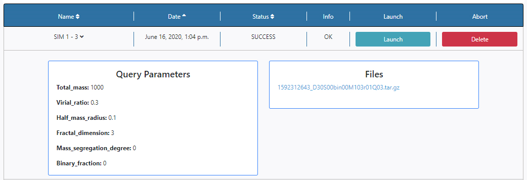
In this case there is one available file, named; 1592312643_D30S00bin00M103r01Q03.tar.gz.
The first number is a unique file identifier, the rest of the characters make reference to the query parameters and hence the contents of the file, use to extract this file.
The file can be downloaded from the Queries Status section or can also be found in the File Manager section of the Data tab. The files are stored under /Home/sources/sim.
Considerations:
Other parameters used to create theses simulations have been:
- Mass function: Kroupa (2001)
- Mass range: (0.1-300) M
- Density profile: Plummer
- Stellar evolution: Eggleton, Tout & Hurley
- Metallicity: Solar (Z=0.02)
- No Galactic tidal field
- Tcritical = 100 Myr
- Output interval = 1.0 Myr
- Primordial binary fraction (Fbin) = 0.0, 0.5 number of binary systems = 0.5 N Fbin
- Pairing is random but separate pairing for components with masses m > Msort
- Msort = 5.0 M
- Semi-major axis distribution: based on Kroupa (1995) period distribution for Msort
- Use period distribution for massive binaries with Mprimary > Msort from Sana & Evans (2011)
- binary star evolution using BSE (Hurley, Tout & Pols 2002)
- Energy-check time step = 0.2 Myr
- Removal of escapers: regular removal at 2*Rtide and output in ESC
- Use random kick velocity and present-day escape velocity to determine retention of compact remnants and evolved binary components
In the location folder of each simulation, there is one folder with the name of the simulation. In this folder the basic information of stars in each time-step is given. There are four types of files:
- *-com (information of the center-of-mass of the multiple systems),
- *-bin (information of the binary systems)
- *-higher (information on the higher-order systems, with more than one companions): The detail of the output of these three types of files are given below.
*-all (information on the single stars in different time-steps), the files contain 12 columns of Name, X, Y, Z, VX, VY, VZ, KSTAR, ZLMSTY, RADIUS, MASS, Ncompanions
- Name: ID of the stars. User can track a star in different time-steps
- X, Y, Z: Position of stars respect to the center-of-mass of the cluster, in Parsec
- VX, VY, VZ: Velocity of stars, in Km/s
- KSTAR: Stellar evolution types
- ZLMSTY: stellar luminosity L/L
- RADIUS: stellar radius R/R
- MASS: stellar mass M/M Ncompanions:
- number of the companions. e.g. 0: single star, 1: binary system, 2 or higher: multiple systems
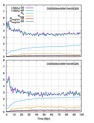
You can use these files to view, for example, different evolutions:
DEAVI provides a File Manager. The File Manager includes a navigation system to interact with the downloaded (query output) or generated files (algorithm output files). The File Manager can be found in the Data tab.

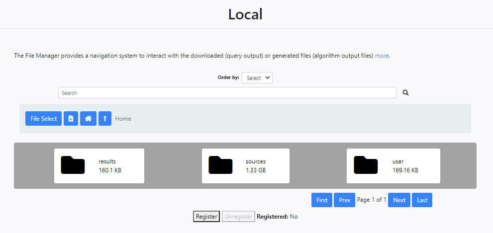
At the very top, the first element of this section consists of a search engine where a certain execution can be located. Next, a series of folders and tools allow navigation in the file manager. Every user has three folders:
- results: This folder contains all the files generated by the algorithms.
- sources: This folder contains in turn three separate folders to hold the files obtained from the Gaia (gaia folder) and Herschel (hsa folder) queries as well as those for the simulations (sim folder).
- user: This folder contains any files uploaded by the user which are needed by the algorithms.
Browsing
The section at the top of the folders panel has several useful features for location and browsing files within all the folders:
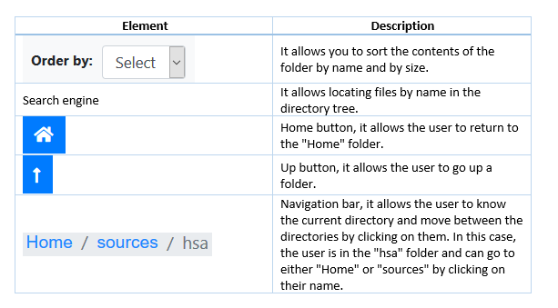
Upload, Download and Delete files
-
Upload files
DEAVI allows the user to upload files in two different ways:
-
Through the web interface of the application. The user has to select the file by clicking on the button,

Then, the user must click on the upload file button,

and the file will be uploaded.
-
Through the SAMP protocol. In this case, the user must first register the hub by clicking on the Register button,

Then, the status will change to Yes and the Unregister button will be activated if the hub is active. Otherwise, the application will inform the user that it has not located the hub,
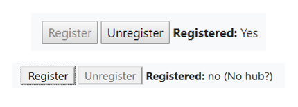
Note that the user must deactivate the mixed content of the web browser used.
-
-
Download and Delete files
When the user views a certain file, its name, its size and the possibility of showing the content, downloading or deleting it are displayed. Below is an example of possible files contained under /Home/sources/gaia,

Show content: When the user clicks on the file name, a new browser window is opened showing its contents.
-
Delete File: If the user clicks on the Delete button,

a pop up will appear reporting that the file will be deleted if the user clicks on Yes. If the user clicks on No, the pop-up window will be closed without deleting the file.
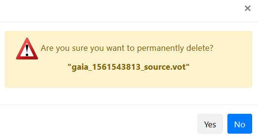
-
Download files: Last, if the user clicks on the Download button,

the file will be downloaded to a local folder.
Both isolated and clustered stars move through space. Their velocities can be measured with respect to different systems: the galaxy, the Sun or the centre of the cluster. The component of stellar motion towards or away from the Sun is known as radial velocity. Proper motion (PM) is the astronomical measure of the observed changes in the apparent places of stars or other celestial objects in the sky when compared to the background of the more distant stars.
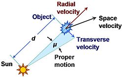
Relation between proper motion and velocity components of an object. (Source: https://en.wikipedia.org/wiki/Proper_motion)
The algorithm Gaia Data Proper Motions is a simple algorithm that queries the Gaia archive for a region of the sky and plots a certain number of stars contained in the results of this query with their proper motions indicated. For this particular tutorial we will use the source NGC 2264 with equatorial coordinates, RA=100.242702, Dec=9.895477.
The input parameters of this algorithm are:

-
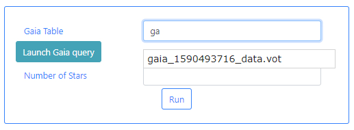
Gaia Table: This is a VOTable file extracted from the Gaia Archive containing information about the stars. This table must exist before the algorithm can be executed. If query files are already available, typing in this field will displayed available files when the typed letters are present in the file names. For example, typing ga, will open a drop-down menu listing those files which containing ga in their name. In the example below one file appears.
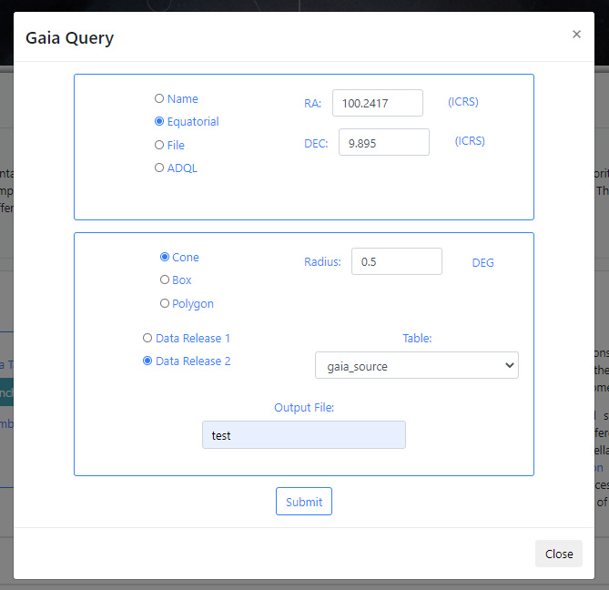
If there are no available query files, the user can make a new query to the Gaia archive by clicking on the Launch Gaia query button. Then, the query form will be displayed. Below is an example query panel where a selection is made in Equatorial coordinates, with a cone radius of 0.5 deg. Searching by Name will resolve the coordinates. The dataset to query is the Gaia Data Release 2 and in particular, the Table gaia_sources within this release. In the field Output File, the name test has been entered. This is important to identify later the results of the query.
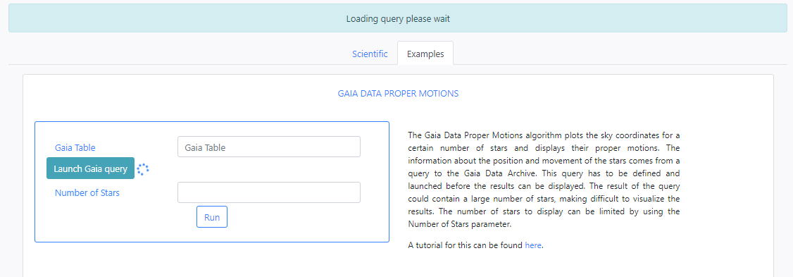
Click Submit to launch the query. Once the query has been launched, an informational message and an animated status icon will appear together with a message saying that the query is being executed.
When the query is finished, the icon will become a "tick" mark.

The status of the query can also be checked in the Status tab of the Queries menu. The name of the file containing the results of the query can also be checked there. In a previous step we had introduced the word test in the Output File of the query form. This has produced a file called: gaia_[unique identifier]_test.vot. Where unique identifier is used to identify different queries. Use the name of this file as input in the Gaia Table parameter field box.
-
Number of stars: Since Gaia queries can contain a large number of stars, this parameter is used to limit the number of stars to include in the plot. This number must be an integer. For the purpose of this tutorial we have introduced 100.
Finally, the user can launch the algorithm by clicking on the Run button.
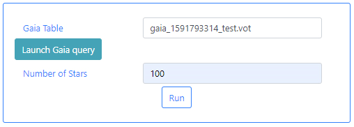
Once launched, the user is redirected to the Pipeline Status section of the Algorithms tab. A message appears saying that the algorithm has started. Also, under the Status column, the message STARTED appears. At this point, the execution can be aborted by clicking the Abort button to the right of the panel.

Once finished, the Status column is changed to SUCCESS if the algorithm has run successfully. At this point, the execution can be deleted by clicking the Delete button to the right of the panel.

By clicking in the arrow close to the name of the algorithm in the Name column, the results panel is opened.
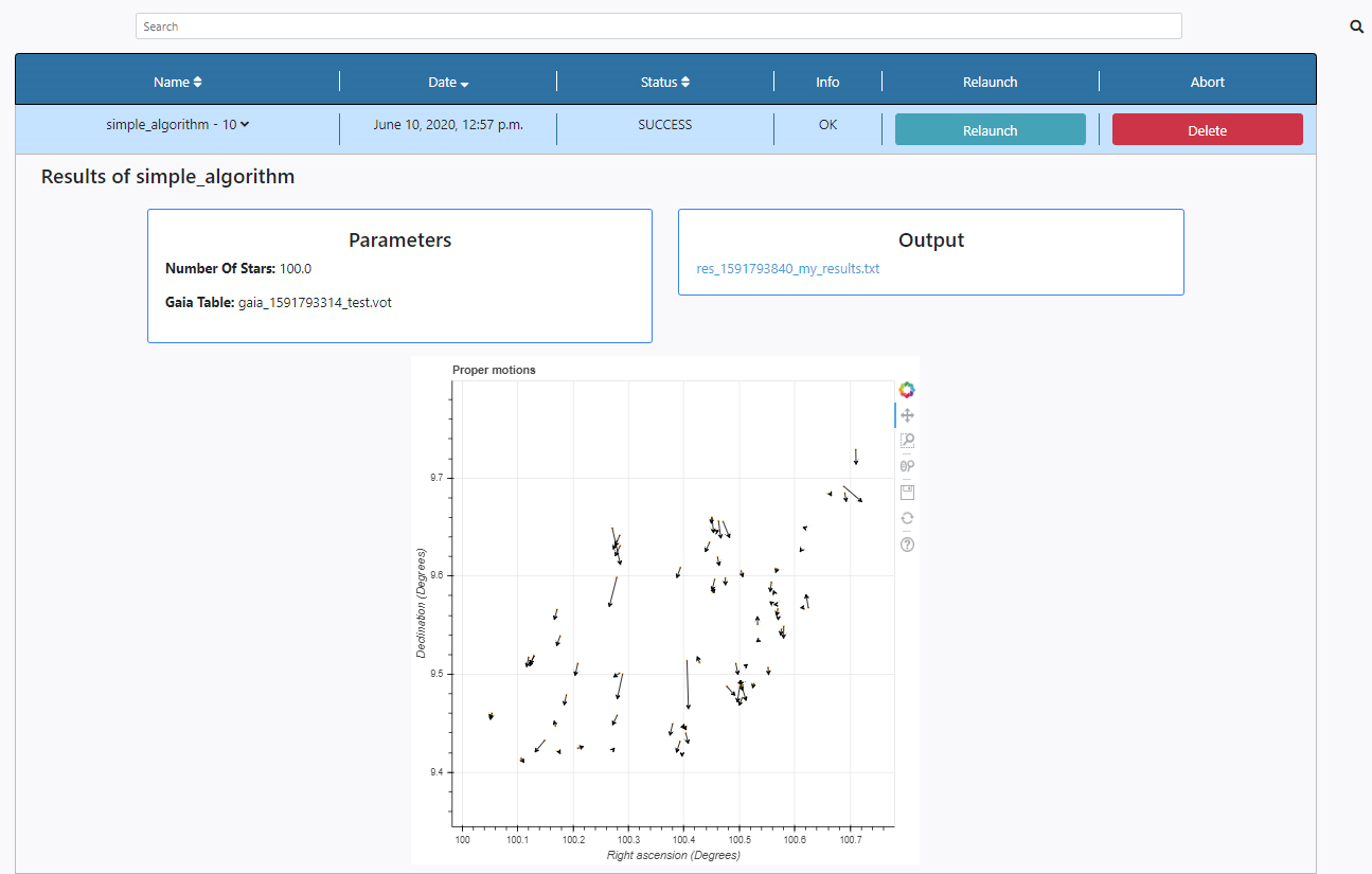
Three panels appear:
- Parameters: here the list of input parameters used in this particular execution of the algorithm is displayed. The results of the query can also be found in the File Manager section of the Data tab. The file is stored under /Home/sources/gaia.
- Output: Any outputs produced by the algorithm are shown here. In this case an ascii file is produce which only contains the number of stars used for plotting. The name of the results file also contains a unique identifier to avoid other executions to overwrite these files. The file name can be clicked to open the file for inspection. The results of the execution can also be found in the File Manager section of the Data tab. The file is stored under /Home/results.
- Plots panel: Any plots produced by the algorithm are displayed here. In this case, the plot contains a representation of stars sky coordinates and arrows indicating the magnitude and direction of the proper motion of the stars. All the plots allow some degree of interaction by using the panel in the top right-hand side. The functionalities allow to zoom, pan and save the plots.
Stars have different colors depending on their surface temperature. This allows the classification of the stars according to their color as listed in the table below.

(Source: https://oneminuteastronomer.com/708/star-colors-explained/)
The Hertzsprung–Russell diagram, abbreviated as H–R diagram, HR diagram or HRD, is a scatter plot of stars showing the relationship between the star’s absolute magnitudes or luminosities versus their stellar classifications or effective temperatures.

(Source: https://en.wikipedia.org/wiki/Luminosity)
The algorithm Wien Law and Hertzsprung-Russell Diagram (HRD) is a simple algorithm that queries the Gaia archive for a region of the sky and makes the two plots above for a certain number of stars contained in the results of this query. For this particular tutorial we will use the source NGC 2264 with equatorial coordinates, RA=100.242702, Dec=9.895477.
The input parameters of this algorithm are:
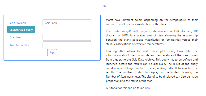
-
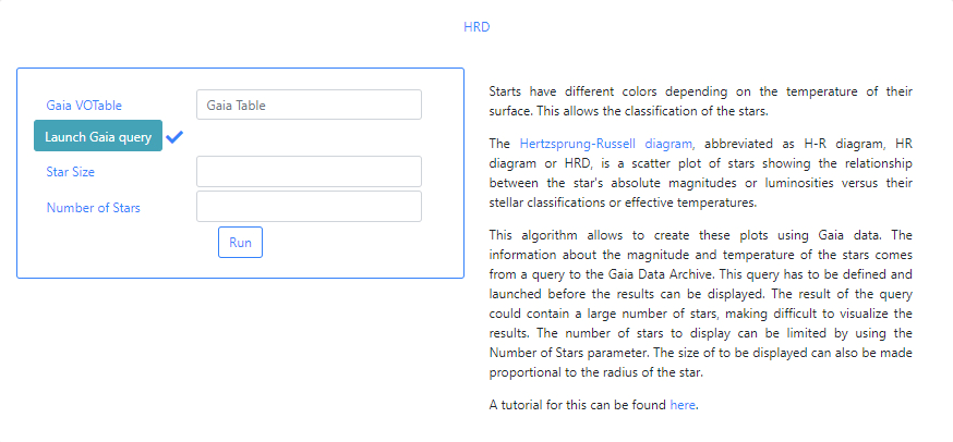
Gaia VOTable: This is a VOTable file extracted from the Gaia Archive containing information about the stars. This table must exist before the algorithm can be executed. If query files are already available, typing in this field will displayed available files when the typed letters are present in the file names. For example, typing ga, will open a drop-down menu listing those files which containing ga in their name. In the example below one file appears.
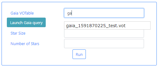
If there are no available query files, the user can make a new query to the Gaia archive by clicking on the Launch Gaia query button. Then, the query form will be displayed. Below is an example query panel where a selection is made in Equatorial coordinates, with a cone radius of 0.5 deg. The dataset to query is the Gaia Data Release 2 and in particular, the Table gaia_sources within this release. In the field Output File, the name test has been entered. This is important to identify later the results of the query.

Click Submit to launch the query. Once the query has been launched, an informational message and an animated status icon will appear together with a message saying that the query is being executed.
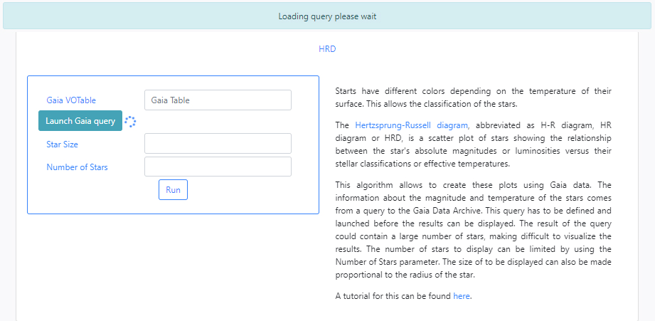
When the query is finished, the icon will become a "tick" mark.
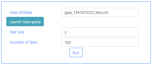
The status of the query can also be checked in the Status tab of the Queries menu. The name of the file containing the results of the query can also be checked there. In a previous step we had introduced the word test in the Output File of the query form. This has produced a file called: gaia_[unique identifier]_test.vot. Where unique identifier is used to identify different queries. Use the name of this file as input in the Gaia Table parameter field box.
-
Star Size: This parameter controls the size of the stars to be plotted. The options are all stars are plotted with equal size, or their size is plotted proportional to their radius (y/n). For the purpose of this tutorial we have introduced y.
-
Number of stars: Since Gaia queries can contain a large number of stars, this parameter is used to limit the number of stars to include in the plot. This number must be an integer. For the purpose of this tutorial we have introduced 100.
Finally, the user can launch the algorithm by clicking on the Run button.
Once launched, the user is redirected to the Pipeline Status section of the Algorithms tab. A message appears saying that the algorithm has started. Also, under the Status column, the message STARTED appears. At this point, the execution can be aborted by clicking the Abort button to the right of the panel.

Once finished, the Status column is changed to SUCCESS if the algorithm has run successfully. At this point, the execution can be deleted by clicking the Delete button to the right of the panel.

By clicking in the arrow close to the name of the algorithm in the Name column, the results panel is opened.
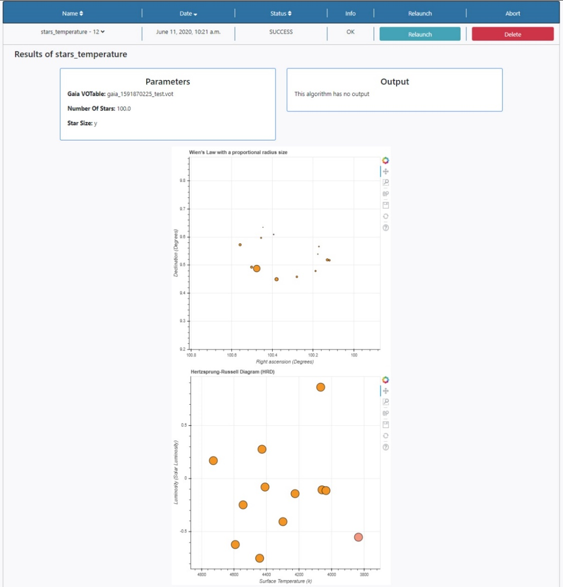
Three panels appear:
- Parameters: here the list of input parameters used in this particular execution of the algorithm is displayed. The results of the query can also be found in the File Manager section of the Data tab. The file is stored under /Home/sources/gaia.
- Output: Any outputs produced by the algorithm are shown here. In this case no output files are produced by this algorithm.
- Plots panel: Any plots produced by the algorithm are displayed here. In this case, two plots are shown, Wien’s Law where the size of the dots is proportional to the radius of the stars, and the HR diagram. All the plots allow some degree of interaction by using the panel in the top right-hand side. The functionalities allow to zoom, pan and save the plots.
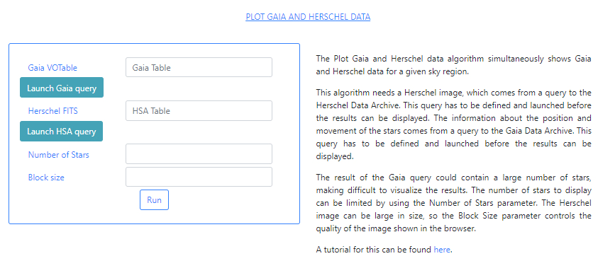
The algorithm Plot Gaia and Herschel Data is a simple algorithm that queries both the Gaia and Herschel archives for a region of the sky. The algorithm plots a certain number of stars contained in the results of the Gaia query, with their proper motions indicated, over the same region of a Herschel image. The input parameters of this algorithm are:
-
Gaia VOTable: This is a VOTable file extracted from the Gaia Archive containing information about the stars. This table must exist before the algorithm can be executed. If query files are already available, typing in this field will displayed available files when the typed letters are present in the file names. For example, typing ga, will open a drop-down menu listing those files which containing ga in their name. In the example below two files appear.
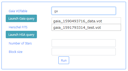
If there are no available query files, the user can make a new query to the Gaia archive by clicking on the Launch Gaia query button. Then, the query form will be displayed. Below is an example query panel where a selection is made in Equatorial coordinates, with a cone radius of 0.5 deg. The dataset to query is the Gaia Data Release 2 and in particular, the Table gaia_sources within this release. In the field Output File the name test has been entered. This is important to identify later the results of the query.

Click Submit to launch the query. Once the query has been launched, an informational message and an animated status icon will appear together with a message saying that the query is being executed.
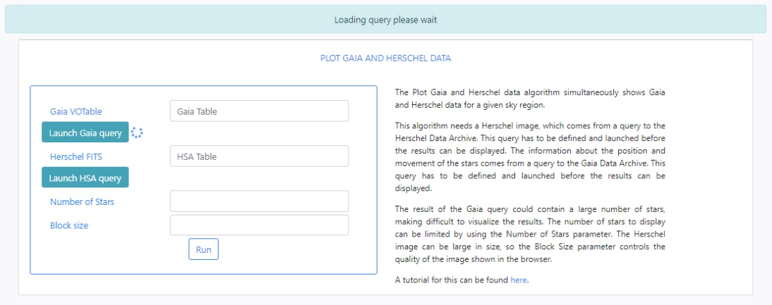
When the query is finished, the icon will become a "tick" mark.
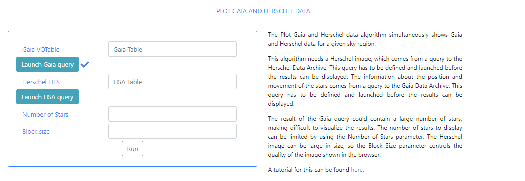
The status of the query can also be checked in the Status tab of the Queries menu. The name of the file containing the results of the query can also be checked there. In a previous step we had introduced the word test in the Output File of the query form. This has produced a file called: gaia_[unique identifier]_test.vot. Where unique identifier is used to identify different queries. Use the name of this file as input in the Gaia Table parameter field box.
-
Herschel FITS: This is a FITS file containing a Herschel image. The image can be extracted from the Herschel Archive. As for the Gaia VOTable field, typing in this field will displayed available files when the typed letters are present in the file names.
If there are no available query files, the user can make a new query to the Herschel archive by clicking on the Launch HSA query button. Then, the query form will be displayed. Below is an example query panel where a selection is made in Equatorial coordinates, with a Cone radius of 0.5 deg. Searching by Name will resolve the coordinates. The image dataset within HSA is queried, in particular, this example works with images from the SPIRE instrument. The level2_5 products are selected from the drop-down menu. In the field Output File, the name test has been entered. This is important to identify later the results of the query.
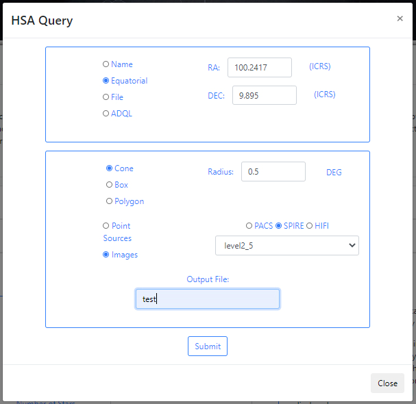
Click Submit to launch the query. Once the query has been launched, an informational message and an animated status icon will appear together with a message saying that the query is being executed. Queries to the HSA archive can take some time to process as the images can be large in size.
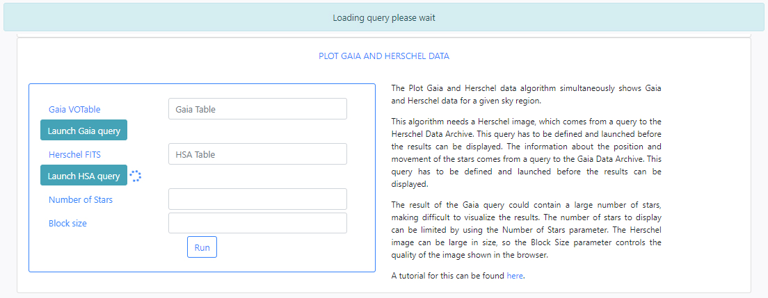
When the query is finished, the icon will become a "tick" mark.
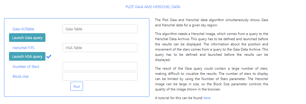
The status of the queries can also be checked in the Status tab of the Queries menu. The names of the files containing the results of the query can also be checked there. In a previous step we had introduced the word test in the Output File of both Gaia and HAS query forms. This has produced a file called: gaia_[unique identifier]_test.vot and a file called . Where unique identifier is used to identify different queries. Use the name of these files as input in the Gaia VOTable and Herschel FITS parameter field box.
- Number of stars: Since Gaia queries can contain a large number of stars, this parameter is used to limit the number of stars to include in the plot. This number must be an integer. For the purpose of this tutorial we have introduced 100.
- Block size: This parameter is used to reduce the quality of the image shown in the browser. This is to optimize loading heavy images. The minimum value is a block size of 1, the original image (maximum quality).
Finally, the user can launch the algorithm by clicking on the Run button. Once launched, the user is redirected to the Pipeline Status section of the Algorithms tab. A message appears saying that the algorithm has started. Also, under the Status column, the message STARTED appears. At this point, the execution can be aborted by clicking the Abort button to the right of the panel.

Once finished, the Status column is changed to SUCCESS if the algorithm has run successfully. At this point, the execution can be deleted by clicking the Delete button to the right of the panel.

By clicking in the arrow close to the name of the algorithm in the Name column, the results panel is opened.
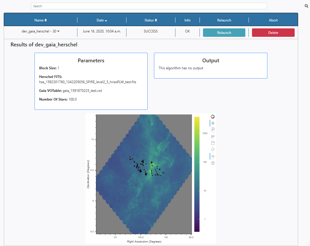
Three panels appear:
- Parameters: here the list of input parameters used in this particular execution of the algorithm is displayed. The results of the queries can also be found in the File Manager section of the Data tab. The files are stored under /Home/sources/gaia and /Home/sources/hsa.
- Output: Any outputs produced by the algorithm are shown here. In this case no output files are produced by this algorithm.
- Plots panel: Any plots produced by the algorithm are displayed here. In this case, the plot contains a representation of starts in sky coordinates and arrows indicating the magnitude and direction of the proper motion of the stars overlay on top of the SPIRE Herschel image. All the plots allow some degree of interaction by using the panel in the top right-hand side. The functionalities allow to zoom, pan and save the plots.
Plotting Gaia data with their proper motions
This algorithm plots the positions of a certain number of stars in a cluster together with their respective proper motions. The input file is a VOTable from the Gaia Archive.
Gaia_pm.py
The first step is to create the Python file where the algorithm is defined. In our case we called it “gaia_pm”.
As usual, we have to import the necessary modules. This algorithm uses Numpy, Astropy, Bokeh and DEAVI libraries.
# Import the necessary modules

                                                        import numpy as np

                                                        from astropy.io.votable import parse

                                                        from avi.utils.plotter import save_plot
                                                        from avi.utils.data.data_file import data_file as data

                                                        from bokeh.plotting import figure, show
                                                        from bokeh.models import Arrow, VeeHead
Next, we create the python class where the algorithm functions are implemented. This class will grow as we add functions. For now,
class Gaia_PM:
Once the class is created, we have to define the inputs. The algorithm will plot a set of stars with their proper motions, so we will need two inputs:
- A VOTable file.
- The number of stars.
class Gaia_PM:
                                                              # Initialize the Gaia table
                                                               gaia_file = ""

                                                              # Starts
                                                               number_stars_displayed = 0.0
In the main class we have to create a “run” function that contains all the tasks to be executed.
class Gaia_PM:
                                                              # Initialize the Gaia table
                                                               gaia_file = ""

                                                              # Starts
                                                               number_stars_displayed = 0.0

                                                               def run(self, id):
                                                               .....
                                                               .....
                                                               .....
- run function:
We will start parsing the data in the VOTable file. Next, we will import the variables of interest. For more information visit the Gaia Data Release Documnetation .
The last step will be to plot the values and save the results. Thus,
"""
Copyright (C) 2016-2020 Quasar Science Resources, S.L.
This file is part of DEAVI.
DEAVI is free software: you can redistribute it and/or modify
it under the terms of the GNU General Public License as published by
the Free Software Foundation, either version 3 of the License, or
(at your option) any later version.
DEAVI is distributed in the hope that it will be useful,
but WITHOUT ANY WARRANTY; without even the implied warranty of
MERCHANTABILITY or FITNESS FOR A PARTICULAR PURPOSE. See the
GNU General Public License for more details.
You should have received a copy of the GNU General Public License
along with DEAVI. If not, see <http://www.gnu.org/licenses/>.
"""
"""
Example 1: This algorithm plots the positions of a certain number of stars in a
cluster together with their respective proper motions. The input file is a VOTable
from the Gaia Archive
"""
# Import the necessary modules
import numpy as np
from astropy.io.votable import parse
from avi.utils.plotter import save_plot
from avi.utils.data.data_file import data_file as data
from bokeh.plotting import figure, show
from bokeh.models import Arrow, VeeHead
class Gaia_PM:
# Initialize the Gaia table
gaia_file = ""
# Starts
number_stars_displayed = 0.0
def run(self, id):
## Gaia VOTABLE
# Extract the information from VOTable file
gaia_data = parse(self.gaia_file)
gaia_list = gaia_data.get_first_table().array
# Parallax obtained from Gaia from the different stars changing units
# from mas to arcseconds
# https://gea.esac.esa.int/archive/documentation/GDR2/Gaia_archive/chap_datamodel/sec_dm_main_tables/ssec_dm_gaia_source.html
paralf = gaia_list['parallax']/1000
# Selection a smaller number of stars (number_stars_displayed)
paralf = paralf[0:self.number_stars_displayed]
# Get the coordinates in the cluster
# Proper motion in declination direction (double, Angular Velocity[mas/year] )
propermot_de_sf= gaia_list['pmdec']
# Proper motion in right ascension direction (double, Angular Velocity[mas/year])
propermot_ra_sf= gaia_list['pmra']
# Declination (double, Angle[deg])
dec_colf = gaia_list['dec']
# Right ascension (double, Angle[deg])
ra_colf = gaia_list['ra']
# Stellar radius (float, Length & Distance[Solar Radius])
radiof = gaia_list['radius_val']
# Creation of an array that will contain only the number of the rows of
# stars with a known PM
starts_with_PM=[]
# Get index of the array with values of PM
for l in range (len(paralf)):
if type(propermot_de_sf[l]) != np.ma.core.MaskedConstant:
starts_with_PM.append(l)
# We initialize the arrays necessary for the subsequent analysis.
propermot_de_sf_new = np.zeros(len(starts_with_PM))
propermot_ra_sf_new = np.zeros(len(starts_with_PM))
dec_colf_new = np.zeros(len(starts_with_PM))
ra_colf_new = np.zeros(len(starts_with_PM))
radiof_new = np.zeros(len(starts_with_PM))
# Function that fills the empty vectors with the real data from Gaia,
# including only the stars with a known proper motion
for j in range(len(starts_with_PM)):
# The proper motions are given in arcseconds per year so they are
# divided by a factor of 3600 to change the units to degrees
propermot_de_sf_new [j]= propermot_de_sf[starts_with_PM[j]]/3600
propermot_ra_sf_new [j]= propermot_ra_sf[starts_with_PM[j]]/3600
dec_colf_new[j] = dec_colf[starts_with_PM[j]]
ra_colf_new[j] = ra_colf[starts_with_PM[j]]
radiof_new[j] = radiof[starts_with_PM[j]]
# Definition of the variables that will be used to plot the coordinates
# of the stars in 2D (right ascension and declination in degrees)
x = ra_colf_new
y = dec_colf_new
# Definition of the variables that will be used to plot the proper
# motions of the stars in 2D in degrees per year (they are multiplied by
# a factor of 10 to make the proportions more visually understandable in
# the plot)
u = propermot_ra_sf_new*10
v = propermot_de_sf_new*10
# Definition of the graph range and selection of an adequate margin
margin = 0.07
max_ra = max(ra_colf_new) + margin
min_ra = min(ra_colf_new) - margin
max_de = max(dec_colf_new) + margin
min_de = min(dec_colf_new) - margin
# Definition of the function that plots the stars and the arrows that
# represent the proper motions
def radvel(x,y,max_ra, min_ra, max_de, min_de):
# Creation of the image
p = figure(title="Proper motions", x_range=(min_ra,max_ra), y_range=(min_de,max_de))
# Creation of the points that represent the stars and their color
p.circle(x, y, color="#FFD700", line_color="#FF8C00" ,radius = 0.001)
# Title of the axis and units
p.xaxis.axis_label = "Right ascension (Degrees)"
p.yaxis.axis_label = "Declination (Degrees)"
# Creation of the arrows of each star representing their proper motions. The color is chosen too.
for k in range (len(x)):
p.add_layout(Arrow(end=VeeHead(size=4), line_color="black", x_start=x[k], y_start=y[k], x_end=x[k]+u[k], y_end=y[k]+v[k]))
save_plot(id, "gaia", p) # open a browser
show(p)
# The function above is called to obtain the wanted graph
p = radvel(x,y,max_ra, min_ra, max_de, min_de)
# Save the results
res = self.number_stars_displayed
my_file = data(id).file("my_results.txt")
my_file.write(str(res))
my_file.close()
Gaia_pm.json
In addition to the python file, we must create the json file to automatically generate the form in DEAVI.
                                                            {"algorithm":{
                                                               "name": "Gaia_PM",
                                                               "view_name": "Gaia Data with their Proper Motions (PM)",
                                                               "description": "<h3>Gaia Data with PM</h3><p>An representation of Gaia data with the proper motions</p>",
                                                               "input":{
                                                                       "input_1":{
                                                                               "name": "gaia_file",
                                                                               "view_name": "Gaia VOTable",
                                                                               "type": "gaia_table"
                                                                       },
                                                                       "input_2":{
                                                                               "name": "number_stars_displayed",
                                                                               "view_name": "Number of stars",
                                                                               "type": "float"
                                                                       }
                                                               }
                                                            }}
Plotting Gaia and Herschel data simultaneously
The last example shows how use Herschel data. In this case, we modify the first example so that the Gaia and Herschel data are displayed simultaneously.
Gaia_Herschel.py
"""
Copyright (C) 2016-2020 Quasar Science Resources, S.L.
This file is part of DEAVI.
DEAVI is free software: you can redistribute it and/or modify
it under the terms of the GNU General Public License as published by
the Free Software Foundation, either version 3 of the License, or
(at your option) any later version.
DEAVI is distributed in the hope that it will be useful,
but WITHOUT ANY WARRANTY; without even the implied warranty of
MERCHANTABILITY or FITNESS FOR A PARTICULAR PURPOSE. See the
GNU General Public License for more details.
You should have received a copy of the GNU General Public License
along with DEAVI. If not, see <http://www.gnu.org/licenses/>.
"""
"""
Example 3: This algorithm plots the positions of a certain number of stars in a
cluster together with their respective proper motions. Also, it plot the Herschel
image in the same coordinates.
"""
# Import the necessary modules
import numpy as np
from astropy.io.votable import parse
from astropy.io import fits
from astropy.wcs import WCS
from astropy.nddata import block_reduce
from bokeh.plotting import figure, show
from bokeh.models import Arrow, VeeHead, LogColorMapper, ColorBar, LogTicker
from avi.utils.plotter import save_plot
from avi.utils.data.data_file import data_file as data
class Gaia_Herschel:
# Initialize the Gaia and Herschel tables
gaia_table = ""
hsa_table = ""
# Starts
number_stars_displayed = 0.0
# Downsample a data array by applying a function to local blocks.
# See http://docs.astropy.org/en/stable/api/astropy.nddata.block_reduce.html
size_block = 1
def run(self,id):
## Herschel FITS
# Load the FITS file with the world coordinate system
herschel = fits.open(self.hsa_table)
# FITS files have some extensions, we separate them
head = herschel[0].header
# The information is located in the extension 1
im = herschel[1].data
# The World Coordinate System information is located in the header so
w = WCS(head)
# In order to define the figure, we need to create two ndarrays
xpx = np.arange(im.shape[1]+1)-0.5
ypx = np.arange(im.shape[0]+1)-0.5
# Now, we create the grid using the previous ndarrays
xlist, ylist = np.meshgrid(xpx,ypx)
# We want a plot in WCS so we need to convert pixels to WCS
ralist, declist= w.all_pix2world(xlist, ylist, 1)
## Gaia VOTABLE
# Extract the information from VOTABLE file
gaia =parse(self.gaia_table)
gaia_list = gaia.get_first_table().array
# Parallax obtained from gaia from the different stars changing units
# from mas to arcseconds
par = gaia_list['parallax']/1000
# Selection a smaller number of stars (number_stars_displayed)
paralf = par[0:self.number_stars_displayed]
# Get the coordinates and proper motions of the stars in the cluster
# https://gea.esac.esa.int/archive/documentation/GDR2/Gaia_archive/chap_datamodel/sec_dm_main_tables/ssec_dm_gaia_source.html
# Proper motion in declination direction (double, Angular Velocity[mas/year] )
propermot_de_sf= gaia_list['pmdec']
# Proper motion in right ascension direction (double, Angular Velocity[mas/year])
propermot_ra_sf= gaia_list['pmra']
# Declination (double, Angle[deg])
dec_colf = gaia_list['dec']
# Right ascension (double, Angle[deg])
ra_colf = gaia_list['ra']
# Stellar radius (float, Length & Distance[Solar Radius])
radiof = gaia_list['radius_val']
# Creation of an array that will contain only the number of the rows of
# stars with a known proper motion (DR2)
starts_with_pm=[]
for l in range (len(paralf)):
if type(propermot_de_sf[l]) != np.ma.core.MaskedConstant:
starts_with_pm.append(l)
# We initialize the arrays necessary for the subsequent analysis.
propermot_de_sf_new = np.zeros(len(starts_with_pm))
propermot_ra_sf_new = np.zeros(len(starts_with_pm))
dec_colf_new = np.zeros(len(starts_with_pm))
ra_colf_new = np.zeros(len(starts_with_pm))
paral_new = np.zeros(len(starts_with_pm))
radiof_new = np.zeros(len(starts_with_pm))
# Function that fills the empty vectors with the real data from gaia,
# including only the stars with a known proper motion
for j in range(len(starts_with_pm)):
# The proper motions are given in arcseconds per year so they are
# divided by a factor of 3600 to change the units to degrees
propermot_de_sf_new [j]= propermot_de_sf[starts_with_pm[j]]/3600
propermot_ra_sf_new [j]= propermot_ra_sf[starts_with_pm[j]]/3600
dec_colf_new[j] = dec_colf[starts_with_pm[j]]
ra_colf_new[j] = ra_colf[starts_with_pm[j]]
paral_new[j] = paralf[starts_with_pm[j]]
radiof_new[j] = radiof[starts_with_pm[j]]
#Definition of the variables that will be used to plot the coordinates
# of the stars in 2D (right ascension and declination in degrees)
x = ra_colf_new
y = dec_colf_new
# Definition of the variables that will be used to plot the proper
# motions of the stars in 2D in degrees per year (they are multiplied by
# a factor of 10 to make the proportions more visually understandable in
# the plot)
u = propermot_ra_sf_new*10
v = propermot_de_sf_new*10
## Herschel's plot
# Reduce the quality of the image to display
small = block_reduce(im, self.size_block)
# When the mouse is moving through the plot, the coordinates will appear
TOOLTIPS=[("(RA,DEC)","($x,$y)"),("Valor","@image")]
# Creation of the image
main_plot = figure(x_range=(ralist.max(),ralist.min()), y_range=(declist.min(), declist.max()), tooltips=TOOLTIPS)
color_mapper = LogColorMapper(palette="Viridis256", low=np.nanmin(im), high=np.nanmax(im))
# Add to the plot the Herschel image
main_plot.image(image=[small], x=ralist.max(), y=declist.min(), dw=(ralist.max()-ralist.min()), dh=(declist.max()-declist.min()), color_mapper=color_mapper)
color_bar = ColorBar(color_mapper=color_mapper, ticker=LogTicker(), label_standoff=12, border_line_color=None, location=(0,0))
main_plot.add_layout(color_bar, 'right')
# Creation of the points that represent the stars and their color
main_plot.circle(x, y, color="#FFD700", line_color="#FF8C00" ,radius = 0.001)
# Creation of the arrows of each star representing their proper motions.
# The color is chosen too
for m in range(len(x)):
main_plot.add_layout(Arrow(end=VeeHead(size=4), line_color="red", x_start=x[m], y_start=y[m], x_end=x[m]+u[m], y_end=y[m]+v[m]))
# Title of the axis and units
main_plot.xaxis.axis_label="Right Ascension (Degrees)"
main_plot.yaxis.axis_label="Declination (Degrees)"
show(main_plot)
save_plot(id, "Gaia y Herschel", main_plot) # open a browser
Gaia_Herschel.json
                                                        {"algorithm":{
                                                           "name":"Gaia_Herschel",
                                                           "view_name":"Plot Gaia and Herschel data",
                                                           "input":{
                                                                   "input_1":{
                                                                           "name":"gaia_table",
                                                                           "view_name":"Gaia VOTable",
                                                                           "type":"gaia_table"
                                                                   },
                                                                   "input_2":{
                                                                    "name":"hsa_table",
                                                                               "view_name":"Herschel FITS",
                                                                               "type":"hsa_table"
                                                                   },
                                                                   "input_3":{
                                                                               "name":"number_stars_displayed",
                                                                               "view_name":"Number of the stars",
                                                                               "type":"float"
                                                                   },
                                                                   "input_4":{
                                                                               "name":"size_block",
                                                                               "view_name":"Size of the block",
                                                                               "type":"integer"
                                                                   }

                                                       }
                                                    }}
Wien’s Law and Hertzsprung-Russell Diagram (HRD)
By slightly modifying the previous algorithm, we can use other characteristics. In this case, we have plotted the Wien’s law and the HDR in two independent figures.
Wien_HRD.py
"""
Copyright (C) 2016-2020 Quasar Science Resources, S.L.
This file is part of DEAVI.
DEAVI is free software: you can redistribute it and/or modify
it under the terms of the GNU General Public License as published by
the Free Software Foundation, either version 3 of the License, or
(at your option) any later version.
DEAVI is distributed in the hope that it will be useful,
but WITHOUT ANY WARRANTY; without even the implied warranty of
MERCHANTABILITY or FITNESS FOR A PARTICULAR PURPOSE. See the
GNU General Public License for more details.
You should have received a copy of the GNU General Public License
along with DEAVI. If not, see <http://www.gnu.org/licenses/>.
"""
"""
Example 2: Wien's Law and Hertzsprung-Russell Diagram (HRD). The input file is a VOTable
from the Gaia Archive
"""
# Import the necessary modules
import numpy as np
from astropy.io.votable import parse
from bokeh.plotting import figure, show
from avi.utils.plotter import save_plot
class Wien_HDR:
# Initialize the Gaia table
gaia_table = ""
# Starts
number_stars_displayed = 0.0
proportional_size = "y"
def run(self,id):
## Gaia VOTABLE
# Extract the information from VOTable file
gaia =parse(self.gaia_table)
gaia_list = gaia.get_first_table().array
# Parallax obtained from gaia from the different stars changing units
# from mas to arcseconds
par = gaia_list['parallax']/1000
# Selection a smaller number of stars (number_stars_displayed)
paralf = par[0:self.number_stars_displayed]
# Get the coordinates in the cluster
# https://gea.esac.esa.int/archive/documentation/GDR2/Gaia_archive/chap_datamodel/sec_dm_main_tables/ssec_dm_gaia_source.html
# Declination (double, Angle[deg])
dec_colf = gaia_list['dec']
# Right ascension (double, Angle[deg])
ra_colf = gaia_list['ra']
# Stellar radius (float, Length & Distance[Solar Radius])
radiof = gaia_list['radius_val']
# Stellar effective temperature (float, Temperature[K])
temperature= gaia_list['teff_val']
# stellar luminosity (float, Luminosity[Solar Luminosity])
luminosity= gaia_list['lum_val']
# Creation of an array that will contain only the number of the rows of
# stars with a known T, radio and luminosity
starts_with_T=[]
# Get index of the array with values of temperature, radio and luminosity
for l in range (len(paralf)):
if (type(temperature[l]) != np.ma.core.MaskedConstant) and (type(radiof [l]) != np.ma.core.MaskedConstant) and (type(luminosity [l]) != np.ma.core.MaskedConstant):
starts_with_T.append(l)
# We initialize the arrays necessary for the subsequent analysis.
dec_colf_new = np.zeros(len(starts_with_T))
ra_colf_new = np.zeros(len(starts_with_T))
temperature_new = np.zeros(len(starts_with_T))
radiof_new = np.zeros(len(starts_with_T))
luminosity_new = np.zeros(len(starts_with_T))
# Function that fills the empty vectors with the real data from gaia,
# including only the stars with a known T
for j in range(len(starts_with_T)):
dec_colf_new[j] = dec_colf[starts_with_T[j]]
ra_colf_new[j] = ra_colf[starts_with_T[j]]
temperature_new[j] = temperature[starts_with_T[j]]
radiof_new[j] = radiof[starts_with_T[j]]
luminosity_new[j] = luminosity[starts_with_T[j]]
# Definition of the variables that will be used to plot the coordinates
# of the stars in 2D (right ascension and declination in degrees)
x = ra_colf_new
y = dec_colf_new
# In order to define the figure, we need some auxiliary values
max_ra = np.max(ra_colf_new)+0.25
min_ra = np.min(ra_colf_new)-0.25
max_de = np.max(dec_colf_new)+0.25
min_de = np.min(dec_colf_new)-0.25
luminosity_new = np.log10(luminosity_new)
min_T = temperature_new.min() - 0.1
max_T = temperature_new.max() + 0.1
min_L = luminosity_new.min() - 0.1
max_L = luminosity_new.max() + 0.1
def wien_law(x, y, temperature_new, min_ra, max_ra, min_de, max_de, radiof_new):
p = figure(title="Wien’s Law with a proportional radius size", x_range=(max_ra, min_ra), y_range=(min_de,max_de))
p.xaxis.axis_label = "Right ascension (Degrees)"
p.yaxis.axis_label = "Declination (Degrees)"
for k in range(len(temperature_new)):
if self.proportional_size == "y":
radiof_new[k] = abs(np.log10(radiof_new[k])/45)
else:
radiof_new[k] = 0.008
# Class O, onized and neutral helium, weakened hydrogen --> blueish
if temperature_new [k] > 31000:
p.circle(x[k],y[k], radius = radiof_new[k], line_color="black", color = "#ADD8E6")
# Class B, Neutral helium, stronger hydrogen --> Blue-white
if temperature_new [k] < 31000 and temperature_new[k] > 9750:
p.circle(x[k],y[k], radius = radiof_new[k], line_color="black", color = "#e6ffff")
# Class A, Stronger hydrogen, ionized metals --> White
if temperature_new [k] < 9750 and temperature_new[k] > 7100:
p.circle(x[k],y[k], radius = radiof_new[k], line_color="black", color = "#ffffff")
# Class F, Weaker hydrogen, ionized metals --> Yellow - White
if temperature_new [k] < 7100 and temperature_new[k] > 5950:
p.circle(x[k],y[k], radius = radiof_new[k], line_color="black", color = "#ffffcc")
# Class G Weak hydrogen, ionized and neutral metals --> Yellowish
if temperature_new [k] < 5950 and temperature_new[k] > 5250:
p.circle(x[k],y[k], radius = radiof_new[k], line_color="black", color = "#ffff66")
# Class K, Weak hydrogen, neutral metals --> Orange
if temperature_new [k] < 5250 and temperature_new[k] > 3950:
p.circle(x[k],y[k], radius = radiof_new[k], line_color="black", color = "#ff9900")
# Class M, Little or no hydrogen, neutral metals, molecules --> Reddish
if temperature_new[k] < 3950 and temperature_new[k] > 2000:
p.circle(x[k],y[k], radius = radiof_new[k], line_color="black", color = "#ff9980")
save_plot(id, "stars_temperature", p)
show(p)
def hertzsprung_russell_diagram(temperature_new, luminosity_new, radiof_new):
p = figure(title="Hertzsprung-Russell Diagram (HRD)", x_range=(max_T, min_T), y_range=(min_L,max_L))
p.xaxis.axis_label = "Surface Temperature (k)"
p.yaxis.axis_label = "Luminosity (Solar Luminosity)"
for k in range(len(temperature_new)):
radiof_new[k] = 25
# Class O, onized and neutral helium, weakened hydrogen --> blueish
if temperature_new [k] > 31000:
p.circle(temperature_new[k],luminosity_new[k], radius = radiof_new[k], line_color="black", color = "#ADD8E6")
# Class B, Neutral helium, stronger hydrogen --> Blue-white
if temperature_new [k] < 31000 and temperature_new[k] > 9750:
p.circle(temperature_new[k],luminosity_new[k], radius = radiof_new[k], line_color="black", color = "#e6ffff")
# Class A, Stronger hydrogen, ionized metals --> White
if temperature_new [k] < 9750 and temperature_new[k] > 7100:
p.circle(temperature_new[k],luminosity_new[k], radius = radiof_new[k], line_color="black", color = "#ffffff")
# Class F, Weaker hydrogen, ionized metals --> Yellow - White
if temperature_new [k] < 7100 and temperature_new[k] > 5950:
p.circle(temperature_new[k],luminosity_new[k], radius = radiof_new[k], line_color="black", color = "#ffffcc")
# Class G, Weak hydrogen, ionized and neutral metals --> Yellowish
if temperature_new [k] < 5950 and temperature_new[k] > 5250:
p.circle(temperature_new[k],luminosity_new[k], radius = radiof_new[k], line_color="black", color = "#ffff66")
# Class K, Weak hydrogen, neutral metals --> Orange
if temperature_new [k] < 5250 and temperature_new[k] > 3950:
p.circle(temperature_new[k],luminosity_new[k], radius = radiof_new[k], line_color="black", color = "#ff9900")
# Class M, Little or no hydrogen, neutral metals, molecules --> Reddish
if temperature_new[k] < 3950 and temperature_new[k] > 2000:
p.circle(temperature_new[k],luminosity_new[k], radius = radiof_new[k], line_color="black", color = "#ff9980")
save_plot(id, "stars_temperature", p)
show(p)
p1 = wien_law(x, y, temperature_new, min_ra, max_ra, min_de, max_de, radiof_new)
p2 = hertzsprung_russell_diagram(temperature_new, luminosity_new, radiof_new)
Wien_HRD.json
                                                        {"algorithm":{
                                                           "name":"Wien_HDR",
                                                           "view_name":"Wien Law and Hertzsprung-Russell Diagram (HRD)",
                                                           "input":{
                                                                       "input_1":{
                                                                                   "name":"gaia_table",
                                                                                   "view_name":"Gaia VOTable",
                                                                                   "type":"gaia_table"
                                                                       },
                                                                       "input_2":{
                                                                               "name":"proportional_size",
                                                                               "view_name":"Size proportional to the radious (y/n)",
                                                                               "type":"string"
                                                                       },
                                                                       "input_3":{
                                                                               "name":"number_stars_displayed",
                                                                               "view_name":"Number of the stars",
                                                                               "type":"float"
                                                                       }
                                                           }
                                                    }}
